Optimization: Economic applications
 Expected return and capital structure
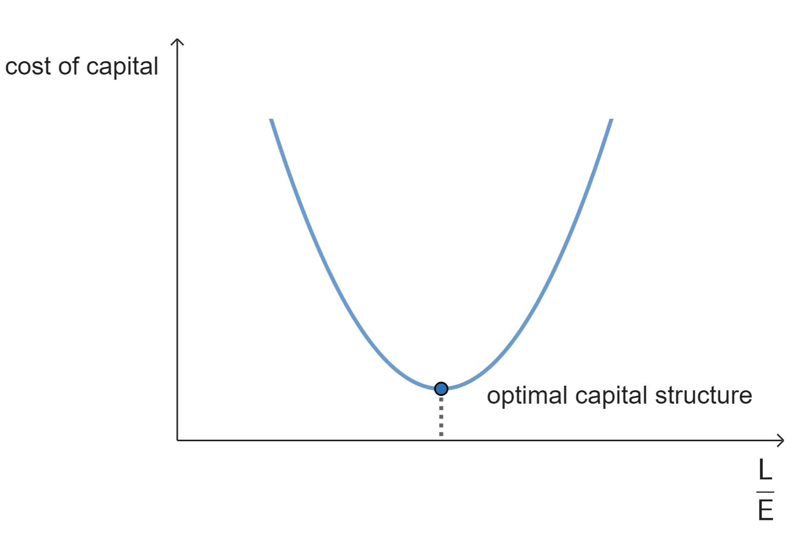
Companies strive to achieve an optimal capital structure. This is a combination of equity and liabilities where the average cost of the company's capital is as low as possible. In general, liabilities are cheaper than equity. This is partly due to the fact that interest paid on borrowed capital is seen as a cost from both a business economics and a tax perspective. At first glance, it seems optimal for a company to attract as much outside capital as possible.
However, attracting large numbers of liabilities also has a downside. This has to do with the role that equity plays within a company. One of the functions of equity is to serve as a buffer that absorbs fluctuations in profit. When a company attracts large numberss of liabilities, this buffer becomes smaller in relative terms. This increases the risk for shareholders and providers of liabilities. To compensate for this increased risk, these investors will demand higher returns, which will increase the costs for the company.
The graph below shows the ratio between liabilities and equity versus the cost of capital. This shows that there is an optimal ratio for a company between liabilities and equity, where the costs of capital are minimised.
Financial leverage formula
The return requirement of capital providers partly depends on the ratio between equity and liabilities. We represent this ratio using the financial leverage formula:
\[ROE = (1-t)(ROA + (ROA – CoD) \cdot \dfrac{L}{E})\]
In the equation, the symbols have the following meaning:
\[\begin{array}{rcl}
t &=& \text{tax rate}\\
ROE &=& \text{return on equity} = \dfrac{\text{net profit}}{\text{equity}}\\
ROA &=& \text{return on assets} = \dfrac{\text{operating income}}{\text{total assets}}\\
CoD &=&\text{cost of debt} = \text{risk-free rate}+\text{risk premium} \cdot \dfrac{L}{E}\\
L &=&\text{market value of liabilities}\\
E &=&\text{market value of equity}\\
\dfrac{L}{E} &=& \text{leverage ratio}\\
\end{array}\]
Factors
The following factors can be distinguished in the leverage formula:
1. The #(1-t)# factor determines the percentage of interest on liabilities that is paid by the company itself. The interest that a company must pay as a result of outstanding liabilities may be offset as costs in the profit and loss account. This provides the company with a tax advantage, which is also called a tax shield.
2. The leverage ratio #\dfrac{L}{E}#. The leverage ratio represents the ratio between liabilities and equity. Highly leveraged companies are characterized by large numbers of liabilities and are generally considered riskier.
3. The interest margin #(ROA – CoD)#. The interest margin is an indication of the difference between the interest on liabilities on the one hand and the return of the company on the other. When the return on liabilities increases, the interest margin will decrease.
4. We call the #(ROA - CoD) \cdot \dfrac{L}{E}# factor the leverage effect.
To find the value of the leverage ratio #{\dfrac{L}{E}}^*# for which the return on equity #ROE# is maximized, we do the following:
\[\begin{array}{rcl}
ROE &=& (1-t) \left(ROA + (ROA - CoD) \cdot \dfrac{L}{E}\right)\\
&&\phantom{xxxxx}\color{blue}{\text{formula for return on equity}}\\
&=& (1-t) \left(ROA + \left(ROA - (\text{risk-free rate} + \text{risk premium} \cdot \dfrac{L}{E} )\right) \cdot \dfrac{L}{E}\right) \\
&&\phantom{xxxxx}\color{blue}{\text{formula for }CoD \text{ filled in}}\\
&=& (1-t) \left(ROA + \left(ROA - (\text{risk-free rate} + \text{risk premium} \cdot x ) \right) \cdot x \right)\\
&&\phantom{xxxxx}\color{blue}{\text{set }\dfrac{L}{E}\text{ equal to } x}\\
&=& (1- 0.40 ) ( 0.100 + ( 0.100 - ( 0.030 + 0.020 \cdot x)) \cdot x)\\
&&\phantom{xxxxx}\color{blue}{\text{substituted values for }t \text{, } ROA \text{, risk-free rate, and risk premium}}\\
&=& 0.6 \cdot ( 0.100 + ( 0.100 x - 0.030 x - 0.020 x^2)\\
&&\phantom{xxxxx}\color{blue}{\text{intermediate step brackets expanded}}\\
&=& 0.06 + 0.06 x - 0.018 x -0.012 x^2\\
&&\phantom{xxxxx}\color{blue}{\text{brackets expanded}}\\
&=& -0.012 x^2 + 0.042 x + 0.06 \\
&&\phantom{xxxxx}\color{blue}{\text{simplified and rewritten}}\\
\end{array}\]
We now have a formula for return on equity in the form #ax^2 + bx + c# with:
- #a = -0.012#
- #b = 0.042#
- #c = 0.060#
\[\begin{array}{rcl}
x_{vertex} &=& -\dfrac{b}{2 a}\\
&&\phantom{xxxxx}\color{blue}{\text{formula for the vertex of a quadratic function}}\\
&=& -\dfrac{0.042}{2\cdot (-0.012)}\\
&&\phantom{xxxxx}\color{blue}{\text{substituted values for }a \text{ and }b }\\
&\approx& 1.75\\
&&\phantom{xxxxx}\color{blue}{\text{calculated}}\\
&\approx& {\dfrac{L}{E}}^*\\
\end{array}\]

Or visit omptest.org if jou are taking an OMPT exam.